Machine Learning Porject 4: Recommendation System
Introduction
This chapter demonstrates a recommendation system using machine learning algorithms.
Recommendation System
When it comes to data science or machine learning, the first thing that crosses our mind is prediction, recommendation systems, or stuff like that. Actually, recommendation systems are pretty common these days. If we talk about some of the most popular websites like Amazon, eBay, and let’s not forget about Facebook, you’ll see those recommendation systems in action. You would definitely have come across something with the tag ‘you might be interested in’, ‘you might know this person’ or ‘people also searched for’ kind of things. So I decided to take a look at how things work and here I am. We’ll talk about some basic and common types of recommendation systems and how they work and will develop them using Python. One thing to be noted; these systems do not match the quality, complexity, or accuracy used by the tech companies but will just give you the idea and a starting point.
Environment Setup
Ipython notebook or now known as a Jupyter notebook is one of the most commonly used techs for scientific computation. The main reason for its usage is because it excels in literate programming. In other words, it has the ability to re-run the portion of a program instead of running the whole which is convenient when dealing with large datasets. The easiest way to get the Jupyter notebook app is installing a scientific Python distribution; the most common of which is Anaconda. You can download the Anaconda distribution from https://www.anaconda.com/download/ and simply install it using default settings for a single user.
Our environment is all set up now so let’s actually do something. Create a new folder naming Book Recommendation System (I named it this way because we are going to build a book recommendation system, but you can name it anything.) Now launch the Anaconda command prompt and start a new notebook by entering the following command.
- $ jupyter notebook
You should see the following screen.
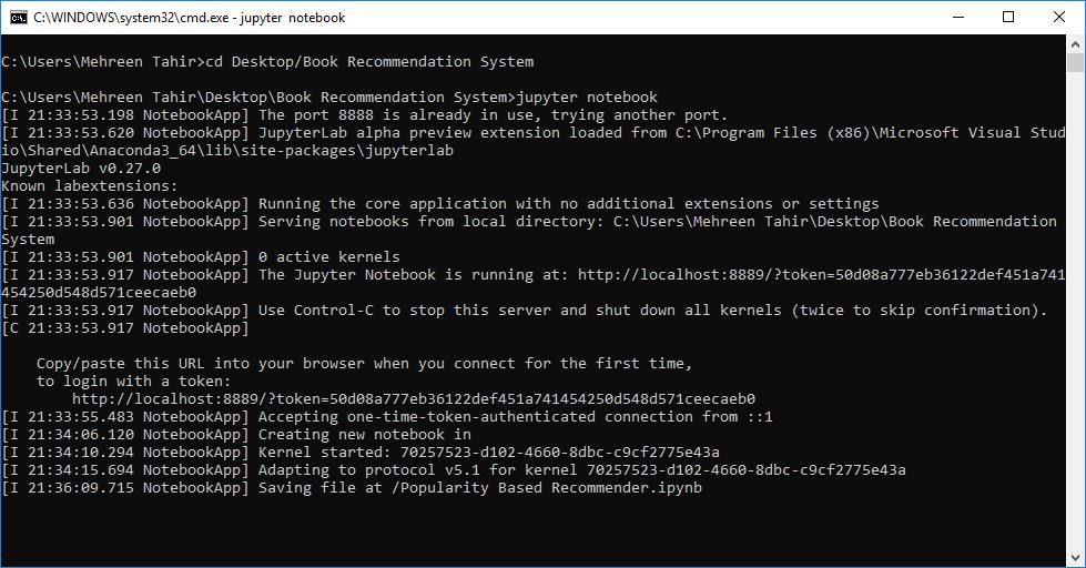
What it did is create an empty notebook inside our mentioned folder and will also launch a web-based interactive environment for you to work in. You can easily rename the file in your browser. Now let’s talk about some commonly used recommendation systems and see things in action.
Popularity based Recommender
This is the most basic recommendation system which offers a generalized recommendation to every user based on the popularity. But it does make sense even with all the simplicity. Let’s take the scenario of an ice cream parlor. Every other customer orders the chocolate flavor so indeed that is more popular among the customers and is a hit of that ice cream parlor. So if a new customer walks in and asks for the best, he would get a suggestion to try the chocolate flavor. The same is true about tourist attractions, hotel recommendations, movies, books, music, etc. whatever is more popular among the general public, is more likely to be recommended to the new customers.
As mentioned before, this type of recommender makes generalized recommendations, not personalized. It means that this system will not take into account the ‘personal’ preferences or choices, rather it would tell you that this particular thing is liked by most of the users.
Building one will clarify the idea behind it. Let’s get started.
- # In[1]:
- #importing libraries
- import pandas as pd
- import numpy as np
Pandas and Numpy are two powerful libraries provided by Python for scientific computation, data manipulation, and data analysis. Numpy; above all; provides high performance, multi-dimensional array along with the tools to manipulate it. Whereas Pandas is known for its data structures and operations for manipulating data.
- # In[2]:
- #reading the files
- data = pd.read_csv('listing.csv', encoding = 'latin-1')
- books = pd.read_csv('books.csv', encoding = 'latin-1')
- # In[3]:
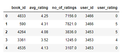
- #use head() function to view first 5 rows for the object based on position. This is just to test if we have right data.
- data.head()

- # In[4]:
- books.head()
- # In[5]:
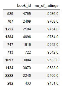
- # Getting recommendation based on No. Of ratings
- rating_count = pd.DataFrame(books, columns=['book_id','no_of_ratings'])
- # Sorting and dropping the duplicates
- rating_count.sort_values('no_of_ratings', ascending=False).drop_duplicates().head(10)
- # In[6]:
- # getting the detail of 5 most rated books
- most_rated_books = pd.DataFrame([4755, 2409, 2194, 4696, 1616], index=np.arange(5), columns=['book_id'])
- detail = pd.merge(most_rated_books, data, on='book_id')
- detail

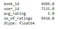
You can also get only the highest-rated books as follows.
- # In[7]:
- # getting the most rated book
- most_rated_book = pd.DataFrame(books, columns=['book_id', 'user_id', 'avg_rating', 'no_of_ratings'])
- most_rated_book.max()
- # In[8]:
- #getting description for most rated book
- most_rated_book.describe()
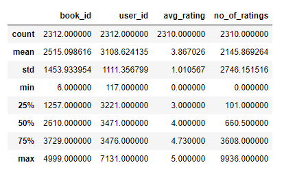
You can also get the description of any column using the same function.
- # In[9]:
- # description for author
- data['author'].describe()
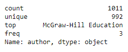
Correlation-Based Recommender
As this is an age of more ‘personalized’ stuff so, popularity based recommenders are not enough to satisfy the need. Thus, there exist Correlation Based Recommenders which would make the recommendations based on the similarity of items (review similarity we’re talking about). The basic idea behind it, being that if you like this item, you are probably going to like an item similar to it. Correlation-Based Recommenders are a simpler form of collaborative filtering based recommenders. They give you more flavor of being personalized as they would recommend the item that is most similar to the item selected before.
We are going to use Pearson’s correlation for our recommendation system. This recommendation system would use item-based similarity; correlate the items based on user ratings.
- # In[1]:
- # importing libraries
- import pandas as pd
- import numpy as np
- # In[2]:
- # reading files
- data = pd.read_csv('listing.csv', encoding = 'latin-1')
- books = pd.read_csv('books.csv', encoding = 'latin-1')
- # In[3]:
- # Checking the data using head function
- books.head()
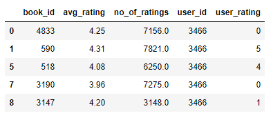
- # In[4]:
- # calculating the mean
- rating = pd.DataFrame(books.groupby('book_id')['no_of_ratings'].mean())
- rating.head()
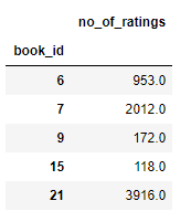
- # In[5]:
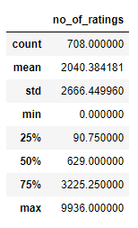
- # getting the description of rating
- rating.describe()
- # In[6]:
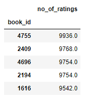
- # sorting based on no of ratings that each book got
- rating.sort_values('no_of_ratings', ascending=False).head()
- # In[7]:
- # Preparing data table for analysis
- ratings_pivot = pd.pivot_table(data=books, values='user_rating', index='user_id', columns='book_id')
- ratings_pivot.head()

As we are interested in finding a correlation between two variables, for that, we are going to use Pearson correlation which would simply measure the linear correlation. In this case, we are interested in knowing the relation between the two books based on user ratings.
- # In[8]:
- correlation_matrix = user_rating.corr(method='pearson')
- correlation_matrix.head(10)
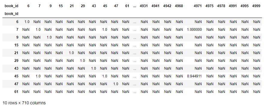
As you can see, now our table contains Pearson correlation coefficient values.
- # In[9]:
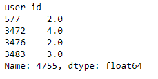
- # getting the users who rated this particular book (most rated) and making sure rating is not zero
- OneManOut_rating = ratings_pivot[4755]
- OneManOut_rating[OneManOut_rating>=0]
Now let's find similar books.
- # In[10]:
- # finding similar books to One Man Out book using Pearson correlation
- similar_to_OneManOut = ratings_pivot.corrwith(OneManOut_rating)
- corr_OneManOut = pd.DataFrame(similar_to_OneManOut, columns=['PearsonR'])
- corr_OneManOut.dropna(inplace=True)
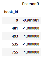
- corr_OneManOut.head()
You’ll encounter a runtime warning because of encountering divide by zero.

But that will not get in our way so it can be ignored. We’ll still get the output as follows.
- # In[11]:
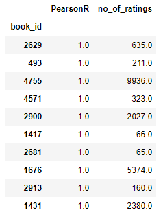
- OneManOut_corr_summary = corr_OneManOut.join(rating)
- # In[12]:
- # getting the most similar book
- OneManOut_corr_summary.sort_values('PearsonR', ascending=False).head(10)
- Building Recommendation Systems In Python
- book_corr_OneManOut = pd.DataFrame([2629, 493, 4755, 4571, 2900, 1417, 2681, 1676, 2913, 1431], index = np.arange(10), columns=['book_id'])
- detail= pd.merge(book_corr_OneManOut, data,on='book_id')
- detail
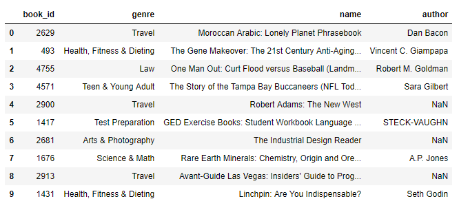
Now if you see the most rated book in our dataset which is One Man Out: Curt Flood Versus Baseball is of the law genre, but our recommendation engine is giving us mixed recommendations including Travel, Law, etc. This is because we are using the relation between ratings to make our recommendation. This book was rated 4 times in our dataset and so was the very first recommended by our recommendation engine. It means our recommender is working.
Content-Base recommender
There exists another type of recommender known as a content-based recommender. This type of recommender uses the description of the item to recommend the next most similar item. Content-based recommenders also make the ‘personalized’ recommendation. The main difference between the correlation-based recommender and content-based recommender is that the former considers the ‘user behavior’ while the latter considers the content for making a recommendation. Content-based recommender uses the product features or keywords used in the description to find the similarity between the items. Let’s see how can we build one.
- # In[1]:
- # importing libraries
- import pandas as pd
- from sklearn.metrics.pairwise import linear_kernel
- from sklearn.feature_extraction.text import TfidfVectorizer
linear_kernelis are used to compute the linear kernel between two variables. We would use this function instead of cosine_similarities() because it is faster and as we are also using TF-IDF vectorization, a simple dot product will give us the same cosine similarity score. Now, what is TF-IDF vector? We cannot compute the similarity between the given description in the form it is in our dataset. This is practically impossible. For this purpose, Term Frequency-Inverse Document Frequency (TF-IDF) is calculated for all the documents which would simply return a matrix with each word representing a column. sklearn’s TfidfVectorizer would do this for us in a couple of lines.
- # In[2]:
- # reading file
- book_description = pd.read_csv('description.csv', encoding = 'latin-1')
- # In[3]:
- # checking if we have the right data
- book_description.head()

- # In[4]:
- # removing the stop words
- books_tfidf = TfidfVectorizer(stop_words='english')
- # filling the missing values with empty string
- book_description['description'] = book_description['description'].fillna('')
- # computing TF-IDF matrix required for calculating cosine similarity
- book_description_matrix = books_tfidf.fit_transform(book_description['description'])
Let's check the shape of our computed matrix.
- # In[5]:
- book_description_matrix.shape

The above shape means that 4186 words are used to describe 143 books in our dataset.
- # In[6]:
- # computing cosine similarity matrix using linear_kernal of sklearn
- cosine_similarity = linear_kernel(book_description_matrix, book_description_matrix)
- # In[7]:
- # Get the pairwise similarity scores of all books compared to the book passed by index, sorting them and getting top 5
- # here 2 is the index of the book in dataset
- similarity_scores = list(enumerate(cosine_similarity[2]))
- similarity_scores = sorted(similarity_scores, key=lambda x: x[1], reverse=True)
- similarity_scores = similarity_scores[1:6]
- # Get the similar books index
- books_index = [i[0] for i in similarity_scores]
- # printingthe top 5 most similar books using integer-location based indexing (iloc)
- print (book_description['name'].iloc[books_index])

Now if we get the recommendation for a book at index 6,

If you notice the results we got; the book at index 2 is similar to the book at index 6 according to our recommendation engine. Let’s follow along with the description and see if our recommender is working.
As per Goodreads; here’s the very short description of the “Angela’s Ashes”,
"When I look back on my childhood I wonder how I managed to survive at all. It was, of course, a miserable childhood: the happy childhood is hardly worth your while. Worse than the ordinary miserable childhood is the miserable Irish childhood, and worse yet is the miserable Irish Catholic childhood."
And “Running with Scissors” goes as,
“The true story of an outlaw childhood where rules were unheard of, the Christmas tree stayed up all year round, Valium was consumed like candy, and if things got dull an electroshock-therapy machine could provide entertainment”.
Which shows somewhat of a similarity between the synopsis of the story. Also, both books belong to the genre ‘Biographies & Memoirs’. This shows that our recommendation is good enough with all its simplicity.
To Readers
The complete repository containing dataset and Jupyter notebooks also exists on GitHub. You can download it here.
Conclusion
So in this chapter, you learned how to build a recommendation system.
Author
Mehreen Tahir
0
6.2k
459.8k
